How to add a passive scalar to your OpenFOAM® simulations
The tutorial Cavity
The Cavity tutorial is part of the icoFoam solver tutorials. The tutorial is located here
$FOAM_TUTORIALS/incompressible/icoFoam/cavity
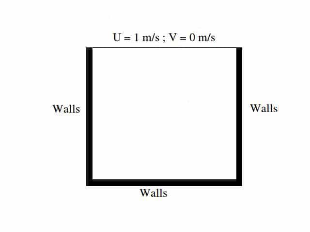
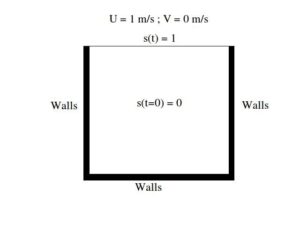
The Cavity tutorial presents the modeling of the flow driven by a moving lid in a square cavity (lid-driven cavity flow). This fluid mechanics problem is a typical validation test case for CFD codes. The problem is considered 2D and the boundary conditions are shown in the figure below. The temporal evolution of the velocity field is also represented.
Reminder about the icoFoam solver
The icoFoam solver of OpenFOAM is an unsteady, incompressible, one phase solver adapted to laminar flows. The solver is based on the PISO loop (and therefore necessarily unsteady). The solver algorithm is described in detail here.
Changing the cavity tutorial - Adding a passive scalar
In order to illustrate the possibility of adding a passive scalar to an OpenFOAM simulation, it is assumed that there is an inert chemical species (called s, for example a rare gas) and modeled by a scalar field whose evolution is governed by the convection / diffusion equation
\(\frac{\partial s}{\partial t} + \overrightarrow{U}\overrightarrow{\nabla s} = \nabla^2 (D s)\)
The concentration of the species is assumed to be zero in the cavity at t = 0 sec and set at 1 on the upper boundary condition representing the moving lid.
The definition of the scalar field is done in the controlDict file located in the /system directory:
{
type scalarTransport;
libs ("libsolverFunctionObjects.so");
enabled true;
writeControl outputTime;
//writeControl timeStep;
//writeInterval 1;
log yes;
nCorr 1;
//difussion coefficient
D 0.0001;
//name of field
field s1;
//use the schemes of field, in this case, U
//schemesField U;</p>
}
scalar2
{
type scalarTransport;
libs ("libsolverFunctionObjects.so");
enabled true;
writeControl outputTime;
//writeControl timeStep;
//writeInterval 1;
log yes;
nCorr 1;
//difussion coefficient
D 0.0005;
//name of field
field s2;
//use the schemes of field, in this case, U
//schemesField U;
}
scalar3
{
type scalarTransport;
libs ("libsolverFunctionObjects.so");
enabled true;
writeControl outputTime;
//writeControl timeStep;
//writeInterval 1;
log yes;
nCorr 1;
//difussion coefficient
D 0.001;
//name of field
field s3;
//use the schemes of field, in this case, U
//schemesField U;
}
In this case, schemesField U being commented the discretization scheme used for the convection term has to to defined in fvScheme the (if not OpenFOAM® uses that defined for U). We choose to use the second order scheme linearUpwind (grad(s) being calculated with the scheme defined in the section gradSchemes, ie a centered scheme).
| ========= | |
| \\ / F ield | OpenFOAM: The Open Source CFD Toolbox |
| \\ / O peration | Version: plus |
| \\ / A nd | Web: www.OpenFOAM.com |
| \\/ M anipulation | |
\*---------------------------------------------------------------------------*/
FoamFile
{
version 2.0;
format ascii;
class dictionary;
location "system";
object fvSchemes;
}
// * * * * * * * * * * * * * * * * * * * * * * * * * * * * * * * * * * * * * //</p>
ddtSchemes
{
default Euler;
}
gradSchemes
{
default Gauss linear;
}
divSchemes
{
default none;
div(phi,U) Gauss linearUpwindV grad(U);
div(phi,s1) Gauss linearUpwind grad(s1);
div(phi,s2) Gauss linearUpwind grad(s2);
div(phi,s3) Gauss linearUpwind grad(s3);
}
laplacianSchemes
{
default Gauss linear orthogonal;
}
interpolationSchemes
{
default linear;
}
snGradSchemes
{
default orthogonal;
}
// ************************************************************************* //
Once the fvSchemes file is correctly adapted, the resolution algorithms of the matrix system need to be set in the fvSolution file:
| ========= | |
| \\ / F ield | OpenFOAM: The Open Source CFD Toolbox |
| \\ / O peration | Version: plus |
| \\ / A nd | Web: www.OpenFOAM.com |
| \\/ M anipulation | |
\*---------------------------------------------------------------------------*/
FoamFile
{
version 2.0;
format ascii;
class dictionary;
location "system";
object fvSolution;
}
// * * * * * * * * * * * * * * * * * * * * * * * * * * * * * * * * * * * * * //</p>
solvers
{
p
{
solver PCG;
preconditioner DIC;
tolerance 1e-06;
relTol 0.05;
}
pFinal
{
$p;
relTol 0.0;
}
U
{
solver smoothSolver;
smoother symGaussSeidel;
tolerance 1e-05;
relTol 0;
}
"s.*"
{
solver PBiCGStab;
preconditioner DILU;
tolerance 1e-08;
relTol 0;
minIter 1;
}
}
PISO
{
nCorrectors 3;
nNonOrthogonalCorrectors 0;
pRefCell 0;
pRefValue 0;
}
// ************************************************************************* //
Finally, it only remains to define the boundary conditions used for the field s by creating a file “s” in the directory /0:
| ========= | |
| \\ / F ield | OpenFOAM: The Open Source CFD Toolbox |
| \\ / O peration | Version: plus |
| \\ / A nd | Web: www.OpenFOAM.com |
| \\/ M anipulation | |
\*---------------------------------------------------------------------------*/
FoamFile
{
version 2.0;
format ascii;
class volScalarField;
object s1;
}
// * * * * * * * * * * * * * * * * * * * * * * * * * * * * * * * * * * * * * //</p>
dimensions [0 0 0 0 0 0 0];
internalField uniform 0;
boundaryField
{
movingWall
{
type fixedValue;
value uniform 1.0;
}
fixedWalls
{
type zeroGradient;
}
frontAndBack
{
type empty;
}
}
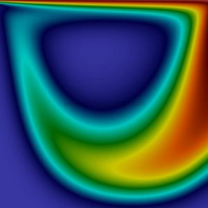
Results
The two images below show the passive scalar evolution for the modified cavity tutorial of OpenFOAM. Two different values of diffusion coefficients are tested:
\(D = 0.0001 m^2/s\) and \( D = 0.0005 m^2/s\)
Conclusions
Download the tutorial (free)
OpenFOAM® tutorial: Passive scalar
0.00€icoFoam solver