Numerical modeling of Rayleigh-Taylor instability with interFoam solver
Introduction
The Rayleigh-Taylor instability is an instability of the interface separating two immiscible fluids ; the densest of which rests on the lightest. Following a disturbance of the interface, the dense fluid enters the light fluid.
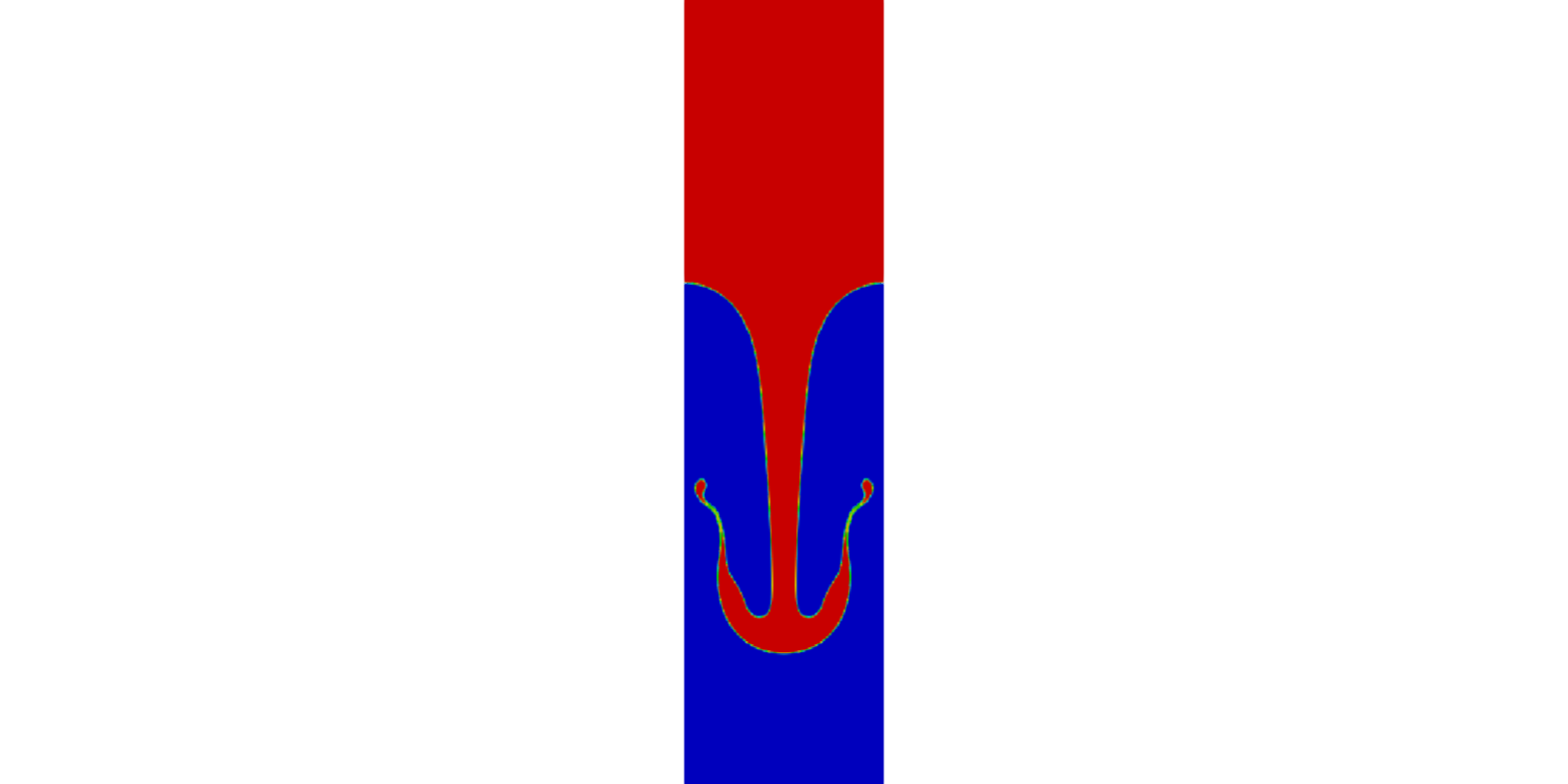
The interface growths with a characteristic “mushroom” shape. For example, Rayleigh-Taylor instability manifests itself in several areas such as astrophysics with the Crab Nebula, thermonuclear fusion with laser implosion of deuterium-tritium targets, or meteorology with cloud formation.
References :
[1] : D.H. SHARP, An overview of Rayleigh-Taylor Instability. 0167-2789/84/$03.00 © Elsevier Science Publishers B.V. (North-Holland Physics Publishing Division)
[2] : Stéphane Popinet. Stabilite et formation de jets dans les bulles cavitantes : developpement d’une methode de chaine de marqueurs adaptee au traitement numerique des equations de navier-stokes avec surfaces libres. http://gfs.sourceforge.net/examples/examples/node7.html
The linear theory
The linear theory describes from Navier-Stokes equations the space and time evolution of the initial interface perturbation. The case is assumed two dimensional and the parameters are shown in the figure below (ref[1]).
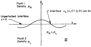
The initial perturbation is defined by the following expression :
\(y_{s} = \eta(t) \cos(kx)\) (1)
It’s possible to show using various arguments from Bernoulli equations or potential theory that the perturbation evolution is described by the following differential equation:
\(\frac{d^2\eta}{dt^2}(t)= \alpha(k)^2\eta(t)\) (2)
With:
\( \alpha(k)^2\ = g(\frac{\rho_{h}-\rho_{l}}{\rho_{h}+\rho_{l}})k-(\frac{\sigma}{\rho_{h}+\rho_{l}})k^3\) (3)
\(\sigma\) being the surface tension (N/m) and\(\rho_{h},\rho_{l}\) the heavier and lighter density.
The differential equation (2) has for solution :
\(\eta(t)=\eta(0)cosh(\alpha t)\) (4)
Numerical setup with OpenFOAM® and interFoam
Geometry, mesh, material properties and boundary condition
The calculation assumptions are those conventionally used (ref [2]) for modeling Rayleigh-Taylor instability.
- The domain size is rectangular 1 m(width)x 4 m(height).
- The mesh is structured (generated with blockMesh) with a cells number of 128×512.
- Lighter fluid properties: density 1.255 kg/m^3 ; dynamic viscosity 3.13 10^-3 Pa.s.
- Heavier fluid properties: density 0.1694 kg/m^3 ; dynamic viscosity 3.13 10^-3 Pa.s.
- Surface tension coefficient : 0.01 N/m.
- Initial perturbation shape (t = 0 sec) : cosinus with 0.05 m of amplitude and 1m of wave lenght.
- Laminar regime.
- Lateral patchs of slip wall type. Upper boundary of “atmosphere” type.
Interface initialization
Setting up the case requires the initialization of the interface between the heavy fluid and the light fluid with a cosine-like shape. There are several possibilities to perform this operation:
- Use swak4Foam: This requires compiling the utility which is not necessarily easy depending on the version of OpenFOAM® you use.
- Use setFields. setFields is an OpenFOAM® utility for initializing a given field, including the possibility to use a stl format surface (generated for example with Salome).
- Use codeStream. codeStream offers the possibility of coding directly in the dictionaries of boundary conditions its instructions.
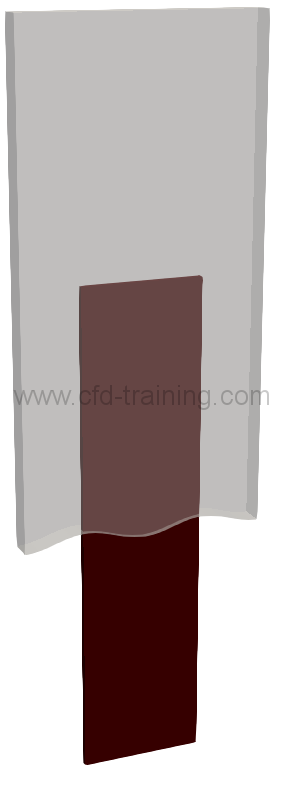
In the context of this post we will limit ourselves to the use of the second method. The use of the setFields command requires the completion of a dictionary located in the /system directory and detailed below:
(
volScalarFieldValue alpha.air 0
);
regions
(
surfaceToCell
{
file "initialVofSurfaceFine.stl";
useSurfaceOrientation false; // use closed surface inside/outside
// test (ignores includeCut,
// outsidePoints)
outsidePoints ((0 -0.5 0.01)); // definition of outside
includeCut false; // cells cut by surface
includeInside true; // cells not on outside of surf
includeOutside false; // cells on outside of surf
nearDistance -1; // cells with centre near surf
// (set to -1 if not used)
curvature 0.9; // cells within nearDistance
// and near surf curvature
// (set to -100 if not used)
fieldValues
(
volScalarFieldValue alpha.air 1
);
}
);
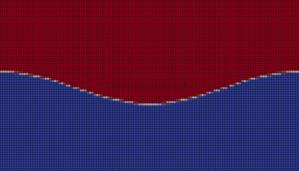
The following figures show initial interface after setFields :

Numerical settings of interFoam
The implementation, respectively, of discretization schemes as well as the settings of the linear solvers are defined respectively in the fvSchemes and fvSolution files:
| ========= | |
| \\ / F ield | OpenFOAM: The Open Source CFD Toolbox |
| \\ / O peration | Version: plus |
| \\ / A nd | Web: www.OpenFOAM.com |
| \\/ M anipulation | |
\*---------------------------------------------------------------------------*/
FoamFile
{
version 2.0;
format ascii;
class dictionary;
location "system";
object fvSchemes;
}
// * * * * * * * * * * * * * * * * * * * * * * * * * * * * * * * * * * * * * //
ddtSchemes
{
default Euler;
}
gradSchemes
{
default Gauss linear;
}
divSchemes
{
div(rhoPhi,U) Gauss linear;
div(phi,alpha) Gauss vanLeer;
div(phirb,alpha) Gauss linear;
div(((rho*nuEff)*dev2(T(grad(U))))) Gauss linear;
}
laplacianSchemes
{
default Gauss linear;
}
interpolationSchemes
{
default linear;
}
snGradSchemes
{
default uncorrected;
}
// ************************************************************************* //
The discretization schemes are second-order except for the temporal derivative scheme (1st implicit order Euler). The term div(phi, alpha) corresponds to the convection term of the transport equation of the volume fraction. The term div(phirb, alpha) corresponds to the second convection term called numerical compression term of interface. This term [3] makes it possible to artificially compress the interface. interFoam solver uses the following numerical equation for the volume fraction:
\(\frac{\partial\alpha}{\partial t} + \nabla (\alpha \overrightarrow{U}) + \nabla (\alpha (1 – \alpha) \overrightarrow{U_r}) \) (5)
The compression effect can be change by adjusting the cAlpha value (which influence the value of the relative speed \(\overrightarrow{U_r}\)) in fvSolution.
- A zero value do not compress the interface \(\overrightarrow{U_r} = \overrightarrow{0}\)(this will lead to a diffusive interface).
- A value of 1 corresponds to a conservative value. In most cases this value is recomended.
- A value greater than one lead to an enhancement of the compression.
It should be noted that this term compression tends to deform the interface.
The pressure / velocity coupling of interFoam is handled through the PISO loop (ie a PIMPLE loop with only one external corrector (nOuterCorrector = 1).
| ========= | |
| \\ / F ield | OpenFOAM: The Open Source CFD Toolbox |
| \\ / O peration | Version: plus |
| \\ / A nd | Web: www.OpenFOAM.com |
| \\/ M anipulation | |
\*---------------------------------------------------------------------------*/
FoamFile
{
version 2.0;
format ascii;
class dictionary;
location "system";
object fvSolution;
}
// * * * * * * * * * * * * * * * * * * * * * * * * * * * * * * * * * * * * * //
solvers
{
"alpha.air.*"
{
nAlphaCorr 3;
nAlphaSubCycles 3;
cAlpha 1;
MULESCorr yes;
nLimiterIter 25;
solver smoothSolver;
smoother symGaussSeidel;
tolerance 1e-10;
relTol 0;
}
"pcorr.*"
{
solver PCG;
preconditioner DIC;
tolerance 1e-7;
relTol 0;
}
p_rgh
{
solver PCG;
preconditioner DIC;
tolerance 1e-7;
relTol 0.0;
}
p_rghFinal
{
$p_rgh;
relTol 0;
}
"U"
{
solver smoothSolver;
smoother symGaussSeidel;
tolerance 1e-08;
relTol 0;
}
"UFinal"
{
$U;
}
}
PIMPLE
{
momentumPredictor no;
nOuterCorrectors 1;
nCorrectors 3;
nNonOrthogonalCorrectors 0;
pRefCell 0;
pRefValue 0;
}
relaxationFactors
{
/*
fields
{
p 0.3;
pFinal 1;
}
equations
{
"U" 0.7;
"UFinal" 1;
}
*/
}
// ************************************************************************* //
interFoam results
The following animated picture show the time evolution of the phase fraction and velocity fields calculated by interFoam. The results show that the perturbation develops downwards generating the “mushroom” characteristic shape.
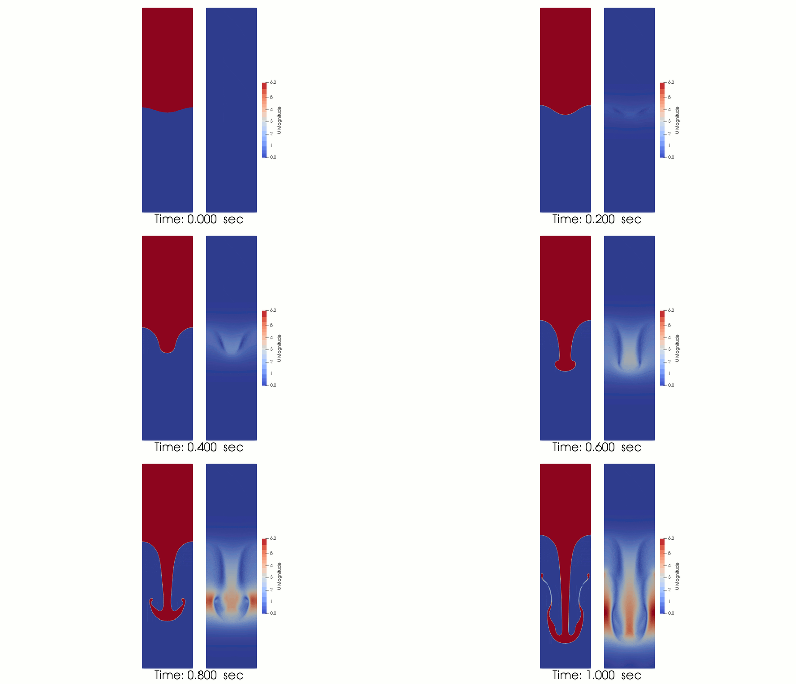
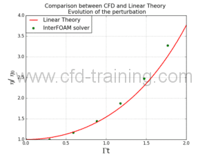
The comparison of interFoam results with linear theory gives reasonable agreement.
