Laminar flow backward facing step flow

The problem of flow in the vicinity of a step is a well-known benchmark for validating CFD codes and estimating the performances of turbulence models. It has the main objective of studying the phenomenon of boundary layer re-attachment. The BFS flow has been studied theoretically, experimentally and numerically by many authors since the 1980s (influence of Reynolds number, thermal, compressibility etc …). The reference experimental data used for the comparison with the numerical results are those of Armaly and Pereira [1], and in particular the laminar case with Reynolds number of 389. The experimental device consists of two rectangular channels with a height of 5.2 mm and 10.1 mm (step height 4.9 mm) in which air circulates at an average speed of 58.63 cm/s..

References :

[1] : B. F. Armaly, Jose c f Pereira, Experimental and Theoretical Investigation of Backward-Facing Step Flow , Journal of Fluid Mechanics · 1983

[2] : Yejun Gong and Franz X. Tanner, Comparison of RANS and LES Models in the Laminar Limit for a Flow Over a Backward-Facing Step Using OpenFOAM, Nineteenth International Multidimensional Engine Modeling Meeting at the SAE Congress April 19, 2009, Detroit, Michigan

The domain of calculation is identical to that used in the study of Gong and Taner [2]. Upstream of the step, the length of the channel is limited to 5 mm. Since experimentally, the velocity profile is fully developed the same profile will be introduced in the calculations. Downstream of the step, the length of the channel is 300 mm.

The dimensions of the computational domain lend themselves perfectly to the use of the blockMesh structured mesher.

The blockMesh utility allows in this case to:    

• create geometry by building blocks from the coordinates of their vertices.
  
• generate a structured mesh by defining the number of nodes for each main direction.
• create the patches for each of the boundary conditions.

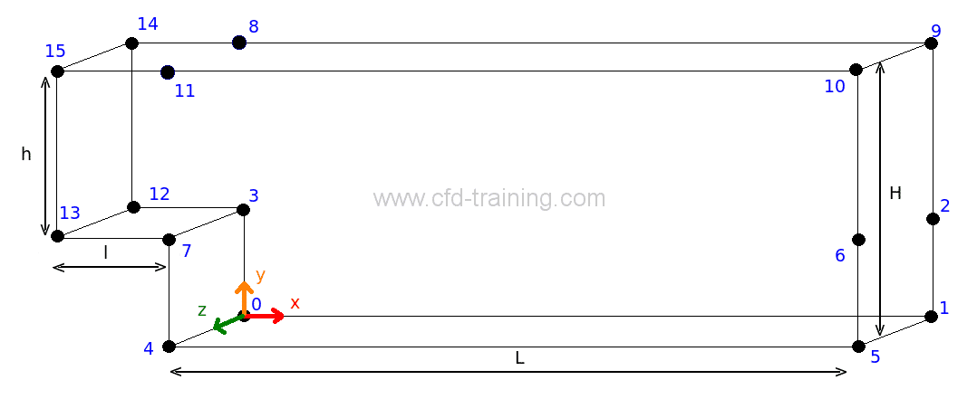
The geometry is divided into three blocks. For this purpose 15 “vertices” are defined in the blockMesh dictionary (directory /system):

[pastacode lang=”cpp” manual=”vertices%0A(%0A%20%20%20%20(0.0%200.0000%200.0)%0A%20%20%20%20(0.3%200.0000%200)%0A%20%20%20%20(0.3%200.0049%200)%0A%20%20%20%20(0.0%200.0049%200)%0A%20%20%20%20(0.0%200.0000%200.005)%0A%20%20%20%20(0.3%200.0000%200.005)%0A%20%20%20%20(0.3%200.0049%200.005)%0A%20%20%20%20(0.0%200.0049%200.005)%0A%0A%20%20%20%20(0.0%200.0101%200)%0A%20%20%20%20(0.3%200.0101%200)%0A%20%20%20%20(0.3%200.0101%200.005)%0A%20%20%20%20(0.0%200.0101%200.005)%0A%0A%20%20%20%20(-0.005%200.0049%200)%0A%20%20%20%20(-0.005%200.0049%200.005)%0A%20%20%20%20(-0.005%200.0101%200)%0A%20%20%20%20(-0.005%200.0101%200.005)%0A)%3B” message=”Vertices declaration” highlight=”” provider=”manual”/]

Computational domain building

A first block (nodes 0 to 7) is used to create the lower part of the channel downstream of the step and a second block (nodes 8 to 11) makes it possible to complete the channel of height 10.1 mm. The last block (nodes 12 3 8 14 13 7 11 15) is used to create the portion of length 5 mm upstream of the step.

[pastacode lang=”cpp” manual=”blocks%0A(%0A%20%20%20%20hex%20(0%201%202%203%204%205%206%207)%20(1000%2040%201)%20simpleGrading%20(%0A(%0A%20%20%20%20(0.25%200.6%201.0)%0A%20%20%20%20(0.75%200.4%2010.0)%0A)%0A(1.0)%20(1.0))%0A%20%20%20%20hex%20(3%202%209%208%207%206%2010%2011)%20(1000%2040%201)%20simpleGrading%20(%0A(%0A%20%20%20%20(0.25%200.6%201.0)%0A%20%20%20%20(0.75%200.4%2010.0)%0A)%0A(1.0)%20(1.0))%0A%20%20%20%20hex%20(12%203%208%2014%2013%207%2011%2015)%20(40%2040%201)%20simpleGrading%20(1.0%201.0%201.0)%0A)%3B” message=”Blocs declaration” highlight=”” provider=”manual”/]

The dictionary has the following lines for creating the non-uniform mesh:

[pastacode lang=”cpp” manual=”simpleGrading%20%0A%20%20%20%20%20%20%20%20(%0A%09%20%20%20(%0A%20%20%20%20%20%20%20%20%20%20%20%20%20%20%20(0.25%200.6%201.0)%20%2F%2F%20Non-uniform%20mesh%20in%20X%0A%20%20%20%20%20%20%20%20%20%20%20%20%20%20%20(0.75%200.4%2010.0)%20%20%2F%2F%20direction%0A%09%20%20%20)%20%0A%09%20%20%20(%0A%20%20%20%20%20%20%20%20%20%20%20%20%20%20%201%20%2F%2FY%20direction%0A%20%20%20%20%20%20%20%20%20%20%20)%0A%09%20%20%20(%0A%20%20%20%20%20%20%20%20%20%20%20%20%20%20%201%20%2F%2FZ%20direction%0A%20%20%20%20%20%20%20%20%20%20%20)%0A%09)” message=”Non-uniform nodes generation” highlight=”” provider=”manual”/]

These lines indicate that in the X direction a non-uniform refinement is imposed with the following characteristics:

• 60% of the total number of meshes is affected, with a growth factor of 1, to 25% of the length of the block.
• 40% of the total number of meshes is affected, with a growth factor of 10, to 75% of the length of the block.

For the other directions (Y and Z) the number of cells is assigned uniformly.

After defining the different nodes necessary for the mesh, the patches of the domain are also created in the blockMesh file:

[pastacode lang=”cpp” manual=”boundary%0A(%0A%20%20%20%20inlet%0A%20%20%20%20%7B%0A%20%20%20%20%20%20%20%20type%20patch%3B%0A%20%20%20%20%20%20%20%20faces%0A%20%20%20%20%20%20%20%20(%0A%20%20%20%20%20%20%20%20%20%20%20%20(12%2013%2014%2015)%0A%20%20%20%20%20%20%20%20)%3B%0A%20%20%20%20%7D%0A%20%20%20%20outlet%0A%20%20%20%20%7B%0A%20%20%20%20%20%20%20%20type%20patch%3B%0A%20%20%20%20%20%20%20%20faces%0A%20%20%20%20%20%20%20%20(%0A%20%20%20%20%20%20%20%20%20%20%20%20(1%205%206%202)%0A%20%20%20%20%20%20%20%20%20%20%20%20(2%206%2010%209)%0A%20%20%20%20%20%20%20%20)%3B%0A%20%20%20%20%7D%0A%20%20%20%20walls%0A%20%20%20%20%7B%0A%20%20%20%20%20%20%20%20type%20wall%3B%0A%20%20%20%20%20%20%20%20faces%0A%20%20%20%20%20%20%20%20(%0A%20%20%20%20%20%20%20%20%20%20%20%20(14%208%2011%2015)%0A%20%20%20%20%20%20%20%20%20%20%20%20(8%209%2010%2011)%0A%20%20%20%20%20%20%20%20%20%20%20%20(12%203%207%2013)%0A%20%20%20%20%20%20%20%20%20%20%20%20(0%204%207%203)%0A%20%20%20%20%20%20%20%20)%3B%0A%20%20%20%20%7D%0A%20%20%20%20frontAndBack%0A%20%20%20%20%7B%0A%20%20%20%20%20%20%20%20type%20empty%3B%0A%20%20%20%20%20%20%20%20faces%0A%20%20%20%20%20%20%20%20(%0A%20%20%20%20%20%20%20%20%20%20%20%20(12%203%208%2014)%0A%20%20%20%20%20%20%20%20%20%20%20%20(3%202%209%208)%0A%20%20%20%20%20%20%20%20%20%20%20%20(0%201%202%203)%0A%20%20%20%20%20%20%20%20%20%20%20%20(13%207%2011%2015)%0A%20%20%20%20%20%20%20%20%20%20%20%20(7%206%2010%2011)%0A%20%20%20%20%20%20%20%20%20%20%20%20(4%205%206%207)%0A%20%20%20%20%20%20%20%20)%3B%0A%20%20%20%20%7D%0A)%3B” message=”Patches definition” highlight=”” provider=”manual”/]

Because the problem is modeled with a two-dimensional flow assumption, out-of-plane patches are defined with an empty type.

The mesh is illustrated (input section, middle and output) in the following figures:

The boundary conditions used are standard:

• Inlet: constant velocity and zero pressure gradient.
• Outlet: Zero velocity gradient and static pressure set to 0 Pa.
• Walls: Zero velocity vector and pressure gradient.
  

For the inlet boundary, the velocity profile is fully developed. It is introduced via the codedFixedValue boundary condition.

[pastacode lang=”cpp” manual=”%20%20%20%20inlet%0A%20%20%20%20%7B%0A%20%20%20%20%20%20%20%20type%20%20%20%20%20%20%20%20%20%20%20%20codedFixedValue%3B%0A%20%20%20%20%20%20%20%20value%20%20%20%20%20%20%20%20%20%20%20uniform%20(0%200%200)%3B%0A%20%20%20%20%20%20%20%20%0A%20%20%20%20%20%20%20%20redirectType%20inletLaminarSquareProfil%3B%0A%20%20%20%20%20%20%20%20code%0A%20%20%20%20%20%20%20%20%23%7B%0A%20%20%20%20%20%20%20%20%20%20%20%20%20const%20fvPatch%26%20boundaryPatch%20%3D%20patch()%3B%20%2F%2Fgeneric%0A%20%20%20%20%20%20%20%20%20%20%20%20%20const%20vectorField%26%20Cf%20%3D%20boundaryPatch.Cf()%3B%20%2F%2Fgeneric%0A%20%20%20%20%20%20%20%20%20%20%20%20%20vectorField%26%20field%20%3D%20*this%3B%20%2F%2Fgeneric%0A%0A%20%20%20%20%20%20%20%20%20%20%20%20%20const%20scalar%20H%09%3D%20%090.0052%3B%20%2F%2F%20definition%20of%20the%20channel%20height%0A%20%20%20%20%20%20%20%20%20%20%20%20%20const%20scalar%20Umax%20%20%3D%20%090.879542893%3B%20%2F%2F%20definition%20of%20the%20maximum%20velocity%0A%0A%20%20%20%20%20%20%20%20%20%20%20%20%20forAll(Cf%2C%20faceI)%20%2F%2F%20loop%20over%20all%20the%20patch%20faces%0A%20%20%20%20%20%20%20%20%20%20%20%20%20%7B%0A%0A%20%20%20%20%20%20%20%20%20%20%20%20%20%20%20%20const%20scalar%20y%20%3D%20Cf%5BfaceI%5D.y()%20-%200.0049%3B%20%2F%2F%20y%20coordinate%20of%20the%20faces%20i%0A%09%09field%5BfaceI%5D%20%3D%20vector(%20Umax%20*(4*y%2FH-4*pow(y%2FH%2C2))%2C%200%2C%200)%3B%20%2F%2F%20define%20velocity%20value%20on%20the%20face%20i%0A%20%20%20%20%20%20%20%20%20%20%20%20%20%7D%0A%0A%20%20%20%20%20%20%20%20%20%23%7D%3B%0A%0A%20%20%20%20%7D” message=”Parabolic inlet velocity” highlight=”” provider=”manual”/]

Learn more about using codedFixedValue : https://cfd-training.com/en/2018/05/07/non-uniform-inlet-profil-with-codedfixedvalue/

The objective of the model is to obtain stabilized flow in order to compare the numerical results with the results of [1]. Since one seeks to obtain a stabilized state, it is advantageous to move towards the solver simpleFoam. Nevertheless in the context of this article it was decided to use the icoFoam solver based on the PISO loop. icoFoam is a transient laminar incompressible solver. The flow will therefore be solved transiently until the steady state is obtained.

The choice of the solver is defined in the controlDict file. The time step is constant during the calculation (deltaT 0.0001;). In practice this value of the time step makes it possible to respect the criterion of stability of the PISO loop (Comax ~ 1).

[pastacode lang=”cpp” manual=”application%20%20%20%20%20icoFoam%3B%0AstartFrom%20%20%20%20%20%20%20startTime%3B%0AstartTime%20%20%20%20%20%20%200%3B%0AstopAt%20%20%20%20%20%20%20%20%20%20endTime%3B%0AendTime%20%20%20%20%20%20%20%20%200.70%3B%0AdeltaT%20%20%20%20%20%20%20%20%20%200.0001%3B%0AwriteControl%20%20%20%20timeStep%3B%0AwriteInterval%20%20%2010%3B%0ApurgeWrite%20%20%20%20%20%200%3B%0AwriteFormat%20%20%20%20%20ascii%3B%0AwritePrecision%20%206%3B%0AwriteCompression%20on%3B%0AtimeFormat%20%20%20%20%20%20general%3B%0AtimePrecision%20%20%206%3B%0ArunTimeModifiable%20true%3B%0AadjustTimeStep%20%20no%3B” message=”controlDict settings” highlight=”” provider=”manual”/]

The numerical schemas (fvSchemes files) are second order with the exception of temporal integration with the use of the first order implicit Euler scheme.

[pastacode lang=”cpp” manual=”ddtSchemes%0A%7B%0A%20%20%20%20default%20%20%20%20%20%20%20%20%20Euler%3B%0A%7D%0AgradSchemes%0A%7B%0A%20%20%20%20%20default%20%20%20%20%20%20Gauss%20linear%3B%20%0A%7D%0AdivSchemes%0A%7B%0A%20%20%20%20default%20%20%20%20%20%20%20%20%20Gauss%20linear%3B%20%20%0A%20%20%20%20div((nuEff*dev2(T(grad(U)))))%20Gauss%20linear%3B%0A%7D%0AlaplacianSchemes%0A%7B%0A%20%20%20%20default%20%20%20%20%20%20%20%20%20Gauss%20linear%20uncorrected%3B%0A%7D%0AinterpolationSchemes%0A%7B%0A%20%20%20%20default%20%20%20%20%20%20%20%20%20linear%3B%0A%7D%0AsnGradSchemes%0A%7B%0A%20%20%20%20default%20%20%20%20%20%20%20%20%20uncorrected%3B%0A%7D” message=”Scheme settings” highlight=”” provider=”manual”/]

Finally the settings of the linear solvers are detailed in the fvSolution file:

• PCG solver for pressure
• smoothSolver for speed.
  
• The speed pressure coupling is iterated twice per time steps (nCorrectors 2;).

[pastacode lang=”cpp” manual=”solvers%0A%7B%0A%20%20%20%20p%0A%20%20%20%20%7B%0A%20%20%20%20%20%20%20%20solver%20%20%20%20%20%20%20%20%20%20PCG%3B%0A%20%20%20%20%20%20%20%20preconditioner%20%20DIC%3B%0A%20%20%20%20%20%20%20%20tolerance%20%20%20%20%20%20%201e-07%3B%0A%20%20%20%20%20%20%20%20relTol%20%20%20%20%20%20%20%20%20%200.05%3B%0A%20%20%20%20%7D%0A%20%20%20%20pFinal%0A%20%20%20%20%7B%0A%20%20%20%20%20%20%20%20%24p%3B%0A%20%20%20%20%20%20%20%20relTol%20%20%20%20%20%20%20%20%20%200%3B%0A%20%20%20%20%7D%0A%20%20%20%20U%0A%20%20%20%20%7B%0A%20%20%20%20%20%20%20%20solver%20%20%20%20%20%20%20%20%20%20smoothSolver%3B%0A%20%20%20%20%20%20%20%20smoother%20%20%20%20%20%20%20%20symGaussSeidel%3B%0A%20%20%20%20%20%20%20%20tolerance%20%20%20%20%20%20%201e-06%3B%0A%20%20%20%20%20%20%20%20relTol%20%20%20%20%20%20%20%20%20%200%3B%0A%20%20%20%20%7D%0A%7D%0APISO%0A%7B%0A%20%20%20%20nCorrectors%20%20%20%20%202%3B%0A%20%20%20%20nNonOrthogonalCorrectors%200%3B%0A%7D” message=”solver settings” highlight=”” provider=”manual”/]

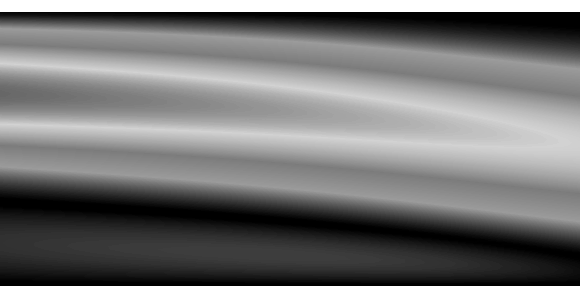
The following figure shows the speed field in the vicinity of the step:

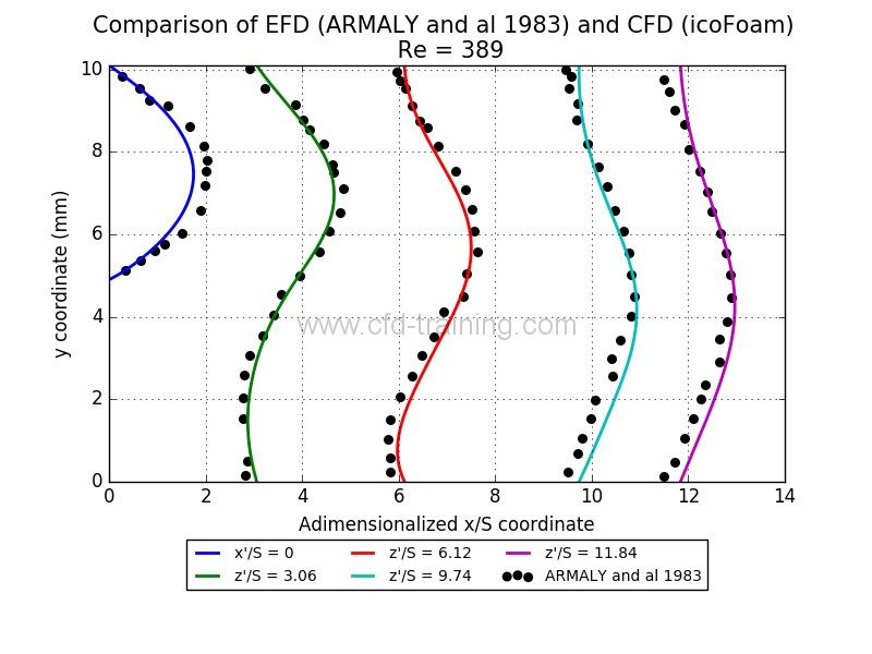
The following figure shows the comparison between standardized speed profiles at different (normalized) distances from the step:

The calculation/measurement agreement is excellent. The calculated velocity profile has the same characteristics as the measured velocity profile. It should be noted that ARMALY et al 1983 indicate that the velocity profile just upstream of walking is not quite parabolic, unlike the boundary condition defined in the numerical model.

This aspect of the modeling explains the deviations of the velocity profile at the step x/s = 0.