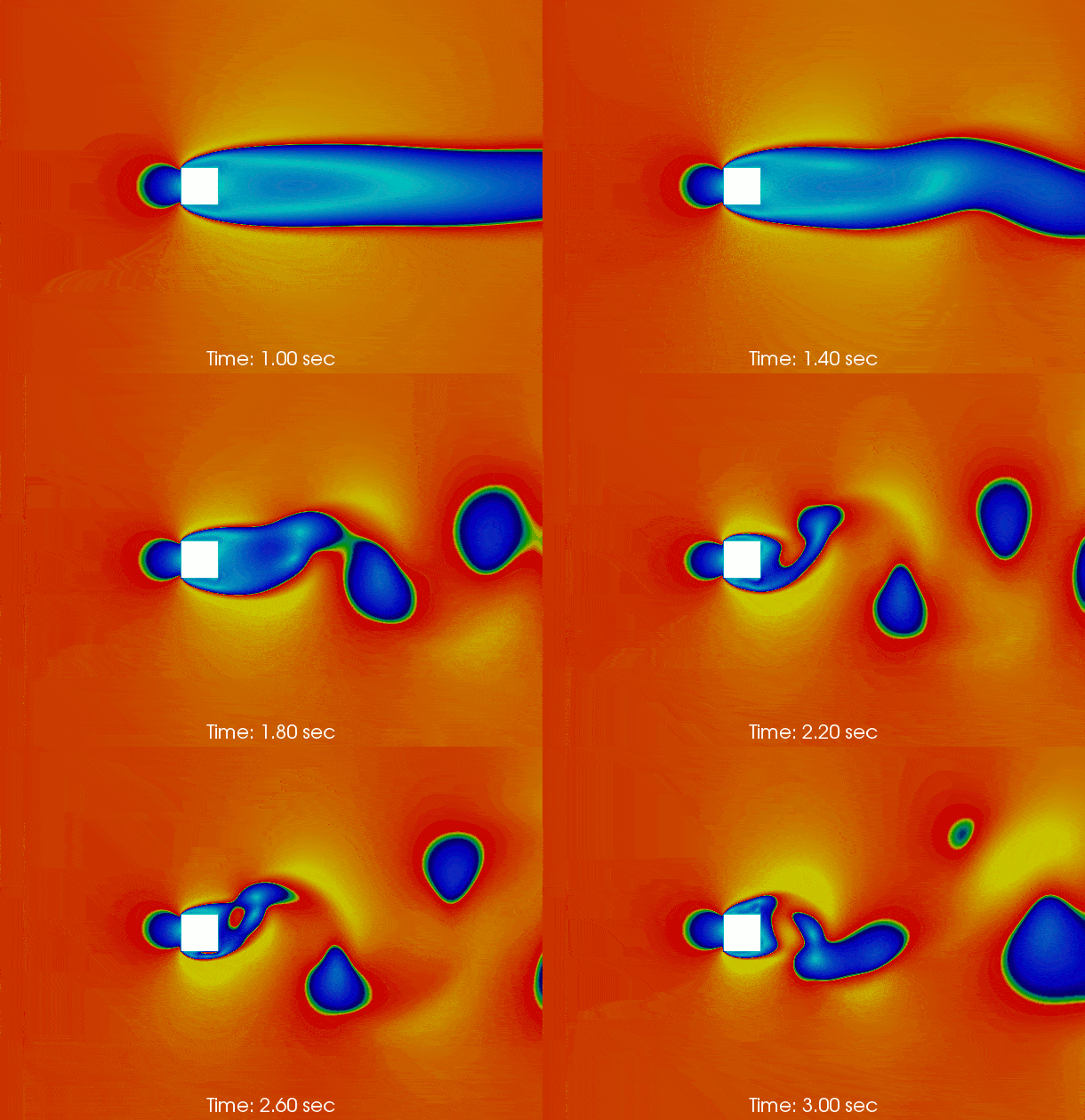
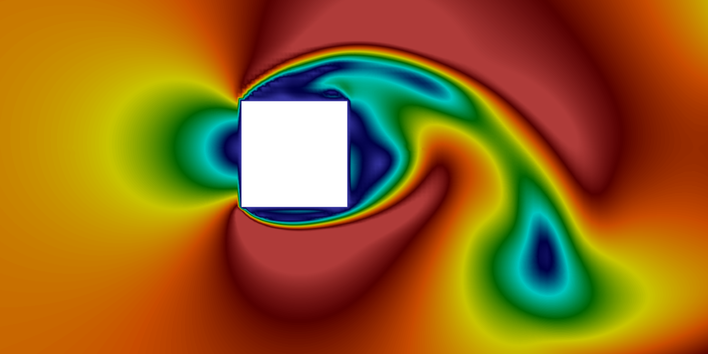
Vortex shedding behind a square with pimpleFoam

Vortex shedding behind a square at Re = 50000

The purpose of this post is to illustrate a vortex shedding application in the case of a square obstacle. The OpenFOAM® solver used is pimpleFoam solver (based on the PIMPLE pressure / velocity coupling algorithm). The mesh is generated with blockMesh and the results are post-processed with paraview.

The Reynolds number of the flow is 50000. The flow velocity is fixed at 5 m/s and the length of the side of the square is 0.1 m. Turbulence is modeled by the URANS equations and the SST (Shear Stress Transport) k-omega turbulence model.

pimpleFoam is a standard solver of OpenFOAM for one phase transient incompressible turbulent (or laminar) flows.

Meshing with blockMesh

The geometry consists of a square of side 0.1 m. This type of geometry, relatively simple, lends itself well to the use of the structured mesher called blockMesh. The use of blockMesh requires to fill a dictionary requiring several entries like:

Node coordinates breaking geometry into blocks
The definition of the different blocks
Patches needed to define the boundary conditions

The figure below shows the geometry with the nodes numbering. Generally with blockMesh it is always advisable to make such a diagram to facilitate the definition of different blocks and patches. The two-dimensional mesh is composed of about 21000 hexahedral cells. Refinement ratios are defined in the X and Y directions to gradually reduce the cell size level near the square walls.

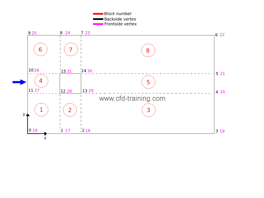
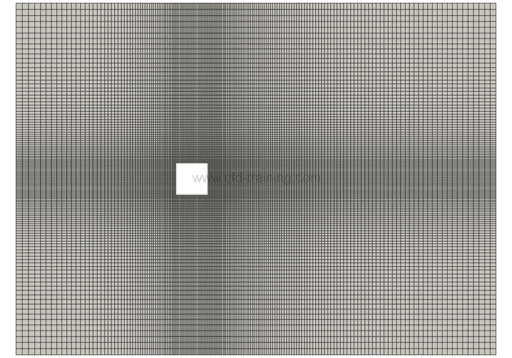
The blockMesh dictionary is written below

/*--------------------------------*- C++ -*----------------------------------*\
| ========= | |
| \\ / F ield | OpenFOAM: The Open Source CFD Toolbox |
| \\ / O peration | Version: plus |
| \\ / A nd | Web: www.OpenFOAM.com |
| \\/ M anipulation | |
\*---------------------------------------------------------------------------*/
FoamFile
{
version 2.0;
format ascii;
class dictionary;
object blockMeshDict;
}

// * * * * * * * * * * * * * * * * * * * * * * * * * * * * * * * * * * * * * //

scale 1;

vertices
(
(0 0 0) //0 vertex number
(0.5 0 0)//1
(0.6 0 0)//2
(1.5 0 0)//3
(1.5 0.5 0)//4
(1.5 0.6 0)//5
(1.5 1.1 0)//6
(0.6 1.1 0)//7
(0.5 1.1 0)//8
(0.0 1.1 0)//9
(0.0 0.6 0)//10
(0.0 0.5 0)//11
(0.5 0.5 0)//12
(0.6 0.5 0)//13
(0.6 0.6 0)//14
(0.5 0.6 0)//15

(0 0 0.05) //16
(0.5 0 0.05)//17
(0.6 0 0.05)//18
(1.5 0 0.05)//19
(1.5 0.5 0.05)//20
(1.5 0.6 0.05)//21
(1.5 1.1 0.05)//22
(0.6 1.1 0.05)//23
(0.5 1.1 0.05)//24
(0.0 1.1 0.05)//25
(0.0 0.6 0.05)//26
(0.0 0.5 0.05)//27
(0.5 0.5 0.05)//28
(0.6 0.5 0.05)//29
(0.6 0.6 0.05)//30
(0.5 0.6 0.05)//31
);

blocks
(
hex (0 1 12 11 16 17 28 27) (50 50 1) simpleGrading (0.2 0.2 1)
hex (1 2 13 12 17 18 29 28) (25 50 1) simpleGrading (1 0.2 1)
hex (2 3 4 13 18 19 20 29) (100 50 1) simpleGrading (5 0.2 1)
hex (11 12 15 10 27 28 31 26) (50 25 1) simpleGrading (0.2 1 1)
hex (13 4 5 14 29 20 21 30) (100 25 1) simpleGrading (5 1 1)
hex (10 15 8 9 26 31 24 25) (50 50 1) simpleGrading (0.2 5 1)
hex (15 14 7 8 31 30 23 24) (25 50 1) simpleGrading (1 5 1)
hex (14 5 6 7 30 21 22 23) (100 50 1) simpleGrading (5 5 1)
);

edges
(
);

boundary
(
inlet
{
type patch;
faces
(
(0 11 27 16)
(11 10 26 27)
(10 9 25 26)
);
}

outlet
{
type patch;
faces
(
(3 4 20 19)
(4 5 21 20)
(5 6 22 21)
);
}

side
{
type patch;
faces
(
(8 9 25 24)
(7 8 24 23)
(6 7 23 22)
(0 1 17 16)
(1 2 18 17)
(2 3 19 18)
);
}

square
{
type wall;
faces
(
(12 15 31 28)
(12 13 29 28)
(13 14 30 29)
(14 15 31 30)
);
}

frontAndBack
{
type empty;
faces
(
(0 1 12 11)
(1 2 13 12)
(2 3 4 13)
(11 12 15 10)
(13 4 5 14)
(10 15 8 9)
(15 14 7 8)
(14 5 6 7)
(16 17 28 27)
(17 18 29 28)
(18 19 20 29)
(27 28 31 26)
(29 20 21 30)
(26 31 24 25)
(31 30 23 24)
(30 21 22 23)
);
}
);

mergePatchPairs
(
);

// ************************************************************************* //

Boundary condition, turbulence model and transport properties

The boundary conditions are conventionally those used for “wind tunnel” simulations with pimpleFoam :

Speed and turbulence quantities imposed at inlet.
Relative pressure imposed at outlet.
Slip wall or symmetry for other patches.
No-slip walls for the boundaries of the square obstacle.

The turbulence model is defined in the turbulenceProperties file. The k-omega SST model has been adopted for this case:

[pastacode lang=”cpp” manual=”simulationType%20%20RAS%3B%0A%0ARAS%0A%7B%0A%20%20%20%20RASModel%20%20%20%20%20%20%20%20kOmegaSST%3B%0A%0A%20%20%20%20turbulence%20%20%20%20%20%20on%3B%0A%0A%20%20%20%20printCoeffs%20%20%20%20%20on%3B%0A%7D” message=”” highlight=”” provider=”manual”/]

Fluid properties are defined in the transportProperties file :

[pastacode lang=”cpp” manual=”transportModel%20%20Newtonian%3B%0A%0Anu%20%20%20%20%20%20%20%20%20%20%20%20%20%201e-05%3B” message=”” highlight=”” provider=”manual”/]

Note that incompressible OpenFOAM® solvers like pimpleFoam solve “p/rho” instead of “p”. That’s why only the kinematic viscosity is required in input data.

Numerical settings - Schemes and linear solvers

The discretization schemes are defined in the fvSchemes file. The mesh quality being very good and the problematic little complex from the numerical point of view it is possible to use directly (without going through first order schemes) second order discretization schemes for spatial derivatives (without limiter). Gradients are evaluated with the centered difference scheme (Gauss linear):

[pastacode lang=”cpp” manual=”gradSchemes%0A%7B%0A%20%20%20%20default%20%20%20%20%20%20%20%20%20Gauss%20linear%3B%0A%7D” message=”” highlight=”” provider=”manual”/]

The calculation of divergence terms is done with second order schemes, linearUpwind and limitedLinear. The limitedLinear scheme is a weighting between upwind and centered difference schemes. If the coefficient is close to 0 the scheme is more accurate but less robust. On the other hand, if the coefficient approaches 1, the opposite happens: the scheme is more stable but less accurate.

[pastacode lang=”cpp” manual=”divSchemes%0A%7B%0A%20%20%20%20default%20%20%20%20%20%20%20%20%20none%3B%0A%20%20%20%20div(phi%2CU)%20%20%20%20%20%20Gauss%20linearUpwind%20grad(U)%3B%0A%20%20%20%20div(phi%2Ck)%20%20%20%20%20%20Gauss%20limitedLinear%201%3B%0A%20%20%20%20div(phi%2Comega)%20%20Gauss%20limitedLinear%201%3B%0A%20%20%20%20div((nuEff*dev2(T(grad(U)))))%20Gauss%20linear%3B%0A%7D” message=”” highlight=”” provider=”manual”/]

The Laplacians discretization requires two inputs: a scheme for the interpolation of the diffusion coefficient (the only possibility is linear ) and a scheme for the normal surface gradient (uncorrected taking into account the quality of the mesh). The interpolation scheme for calculating the values of the faces knowing the values at the cell centers is linear.

[pastacode lang=”cpp” manual=”laplacianSchemes%0A%7B%0A%20%20%20%20default%20%20%20%20%20%20%20%20%20Gauss%20linear%20uncorrected%3B%0A%7D%0A%0AinterpolationSchemes%0A%7B%0A%20%20%20%20default%20%20%20%20%20%20%20%20%20linear%3B%0A%7D%0A%0AsnGradSchemes%0A%7B%0A%20%20%20%20default%20%20%20%20%20%20%20%20%20uncorrected%3B%0A%7D” message=”” highlight=”” provider=”manual”/]

Finally the wall distance is computed using the meshWave method:

[pastacode lang=”cpp” manual=”wallDist%0A%7B%0A%20%20%20%20method%20meshWave%3B%0A%7D%0A” message=”” highlight=”” provider=”manual”/]

In the controlDict file the initial time step is set to 10^-5 sec. For the rest of simulation the time step is automatically determined by the solver according to a maximal Courant Number criterion of 0.9.

[pastacode lang=”cpp” manual=”deltaT%20%20%20%20%20%20%20%20%20%201e-5%3B%0A%0AadjustTimeStep%20%20yes%3B%0A%0AmaxCo%20%20%20%20%20%20%20%20%20%20%200.9%3B” message=”” highlight=”” provider=”manual”/]

Linear solvers are set in the fvSolution file. For linear solvers, OpenFOAM® offers many possibilities. As part of this simulation the following settings have been adopted:

a GAMG solver with GaussSeidel smoother for pressure (symmetric matrix).
a smoothSolver type solver with a symGauddSeidel type smoother for the transport variables (k, omega, U) (antisymmetric matrix).

Note that it is also possible to use a PBiCGStab type solver with a DILU pre-conditioner for the transport variables (k, omega, U) or a PCG solver for the pressure.

[pastacode lang=”cpp” manual=”solvers%0A%7B%0A%0A%20%20%20%20p%0A%20%20%20%20%7B%0A%20%20%20%20%20%20%20%20solver%20%20%20%20%20%20%20%20%20%20%20GAMG%3B%0A%20%20%20%20%20%20%20%20smoother%20%20%20%20%20%20%20%20%20GaussSeidel%3B%0A%20%20%20%20%20%20%20%20tolerance%20%20%20%20%20%20%20%201e-8%3B%0A%20%20%20%20%7D%0A%0A%20%20%20%20pFinal%0A%20%20%20%20%7B%0A%20%20%20%20%20%20%20%20%24p%3B%0A%20%20%20%20%20%20%20%20tolerance%20%20%20%20%20%20%20%201e-8%3B%0A%20%20%20%20%7D%0A%0A%20%20%20%20%22(U%7Ck%7Comega)%22%0A%20%20%20%20%7B%0A%20%20%20%20%20%20%20%20solver%20%20%20%20%20%20%20%20%20%20smoothSolver%3B%0A%20%20%20%20%20%20%20%20smoother%20%20%20%20%20%20%20%20symGaussSeidel%3B%0A%20%20%20%20%20%20%20%20tolerance%20%20%20%20%20%20%201e-07%3B%0A%20%20%20%20%7D%0A%0A%20%20%20%20%22(U%7Ck%7Comega)Final%22%0A%20%20%20%20%7B%0A%20%20%20%20%20%20%20%20%24U%3B%0A%20%20%20%20%20%20%20%20tolerance%20%20%20%20%20%20%201e-07%3B%0A%20%20%20%20%7D%0A%7D” message=”” highlight=”” provider=”manual”/]

Pressure velocity coupling is handled with PIMPLE algorithm of pimpleFoam. Per time step, 5 external loops and one internal loop are defined. The following link provides some very good practices for the PIMPLE algorithm : https://openfoamwiki.net/index.php/OpenFOAM_guide/The_PIMPLE_algorithm_in_OpenFOAM.

[pastacode lang=”cpp” manual=”PIMPLE%0A%7B%0A%20%20%20%20nOuterCorrectors%20%20%20%205%3B%0A%20%20%20%20nCorrectors%20%20%20%20%20%20%20%20%201%3B%0A%20%20%20%20nNonOrthogonalCorrectors%200%3B%0A%7D” message=”” highlight=”” provider=”manual”/]

Mesh non-orthogonality is zero. Thus, no non-orthogonal correction are required.

Results

The following gif shows the temporal evolution of the flow field calculated by pimpleFoam. The flow instability inducing vortex sheeding is clearly shown.

Conclusions

This brief post has shown how to model the external flow field around a square obstacle. The various stages of the implementation of the numerical model were discussed with an emphasis on numerical settings.