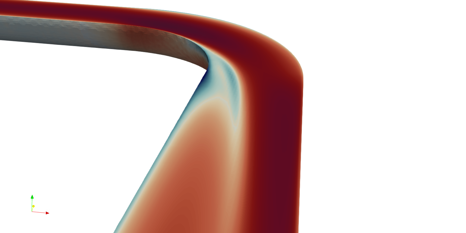
Turbulent flow in a 90° bend
References
[1] : K. Sudo, M. Sumida, H. Hibara – Experimental investigation on turbulent flow in a circular-sectioned 90-degree bend. Experiments in Fluids 25 (1998) 42—49 ( Springer-Verlag 1998 )
paper link : https://link.springer.com/article/10.1007/s003480050206.
Geometry
The diameter of the pipe studied is d = 104 mm. The curvature radius of the elbow is Rc = 208 mm (2d). Experimentally the lengths of the straight sections upstream and downstream of the elbow are respectively 100d and 40d. The line is supplied with air (temperature and atmospheric pressure) at 8.7 m/s (Reynolds number 60000). The 3D model is made under Salome and exported in stl format. The upstream and downstream portions of the elbow are limited to 50d and 20d (which is sufficient here to obtain a fully developed flow).
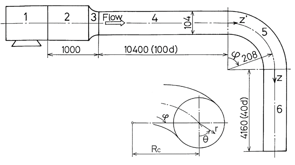
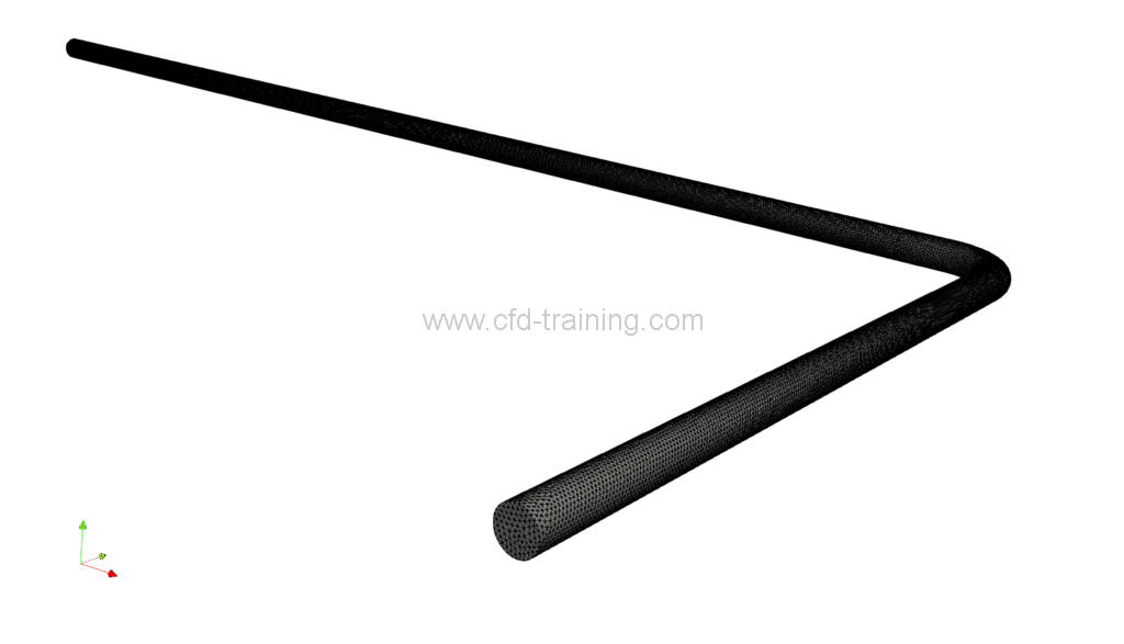
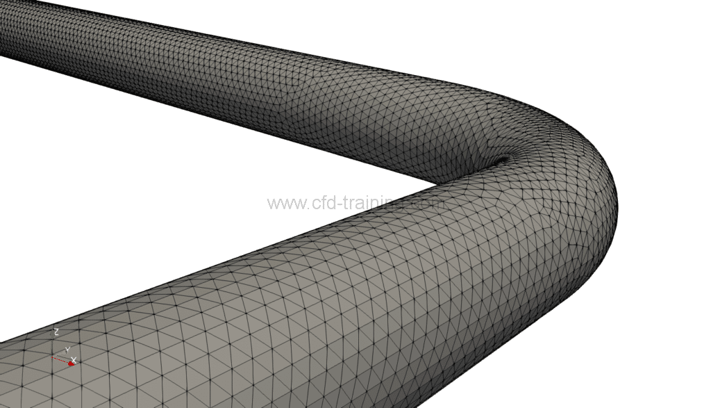
Figure 1 : Experimental device (Sudo et al 1998), (left) – Salome stl surface (center and right)
Mesh
The mesh of level 0 or background mesh (generated with blockMesh) is used to intersect the surface (.stl) of the pipe respectively at the the median plane, the entry plane and exit thus generating the patches of symmetry, input and output of the computational domain.
The mesh of the pipe is generated with snappyHexMesh starting from the “background” mesh. Boundary layer elements are inserted in the near wall region to capture the parietal gradients. The average value of the y+ obtained is 30 (first element located in the log area). In addition, the snappyHexMesh distance mode is used to refine the cells according to the distance to a given patch (here, the wall), which makes it possible to significantly improve the insertion of the boundary layer elements. Finally a refinement block is defined at the elbow region.
The total number cells is 1.1M. No error is detected by the checkMesh utility.
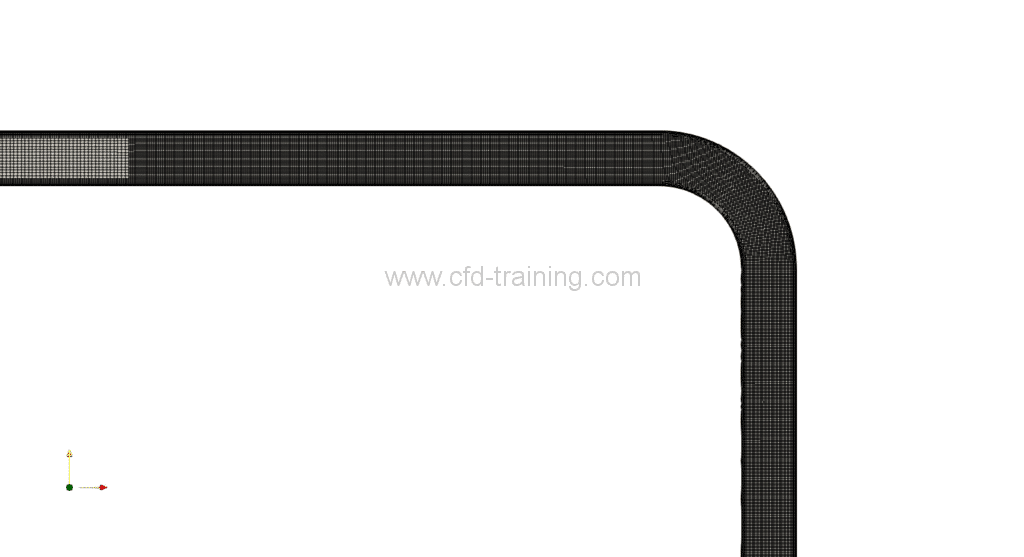
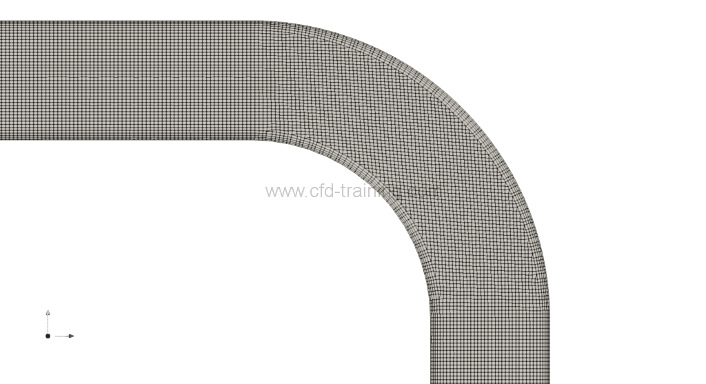
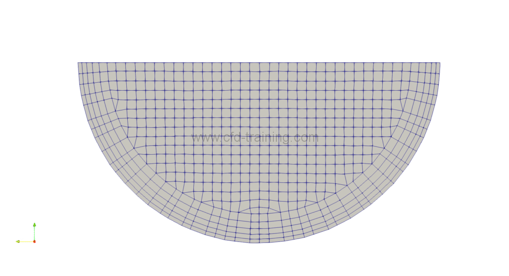
Figure 2 : Cartesian mesh – Mean y+ ~ 30
Boundary conditions
The following table resumes the boundary condition used for the numerical model:
| U | k | epsilon | p | nut | |
|---|---|---|---|---|---|
| Inlet patch | fixedValue (8.7 m/s) | fixedValue | fixedValue | zeroGradient | calculated |
| Outlet pach | zeroGradient | zeroGradient | zeroGradient | fixedValue 0 | calculated |
| Wall patch | noSlip | kqRWallFunction | epsilonWallFunction | zeroGradient | nutkWallFunction |
| Symmetry patch | symmetry | symmetry | symmetry | symmetry | symmetry |
Note that the kqRWallFunction boundary condition is equivalent to a zeroGradient condition.
For k and epsilon assessment the reader is invited to read the Turbulent boundary conditions calculator.
Numerical settings
Schemes
2nd order schemes are used for gradient and divergence (linear and linearUpwind keyword under OpenFOAM®). The Laplacian operator is also discretized with a centered difference type scheme.
| ========= | |
| \\ / F ield | OpenFOAM: The Open Source CFD Toolbox |
| \\ / O peration | Version: v1606+ |
| \\ / A nd | Web: www.OpenFOAM.com |
| \\/ M anipulation | |
\*---------------------------------------------------------------------------*/
FoamFile
{
version 2.0;
format ascii;
class dictionary;
object fvSchemes;
}
// * * * * * * * * * * * * * * * * * * * * * * * * * * * * * * * * * * * * * //
ddtSchemes
{
default steadyState;
}
gradSchemes
{
default Gauss linear;
}
divSchemes
{
div(phi,U) Gauss linearUpwind grad(U);
div(phi,k) Gauss linearUpwind grad(k);
div(phi,epsilon) Gauss linearUpwind grad(epsilon);
div((nuEff*dev2(T(grad(U))))) Gauss linear;
}
laplacianSchemes
{
default Gauss linear corrected;
}
interpolationSchemes
{
default linear;
}
snGradSchemes
{
default corrected;
}
wallDist
{
method meshWave;
}
// ************************************************************************* //
Pressure velocity coupling
The solver used is the simpleFoam solver (incompressible monophasic flow) based on the SIMPLE loop (Semi-Implicit Method for Pressure-Linked Equations). For the presented study, the consistent option is enabled to use the SIMPLEC loop. The SIMPLEC loop has the advantage over the standard SIMPLE loop of being more robust and faster. The numerical model being robust due to the mesh quality non-orthogonal corrector are not necessary. In addition, to facilitate the simpleFoam convergence relaxation factors are introduced.
| ========= | |
| \\ / F ield | OpenFOAM: The Open Source CFD Toolbox |
| \\ / O peration | Version: v1606+ |
| \\ / A nd | Web: www.OpenFOAM.com |
| \\/ M anipulation | |
\*---------------------------------------------------------------------------*/
FoamFile
{
version 2.0;
format ascii;
class dictionary;
object fvSolution;
}
// * * * * * * * * * * * * * * * * * * * * * * * * * * * * * * * * * * * * * //
solvers
{
p
{
solver GAMG;
tolerance 1e-7;
relTol 0.01;
smoother GaussSeidel;
nPreSweeps 0;
nPostSweeps 2;
cacheAgglomeration on;
agglomerator faceAreaPair;
nCellsInCoarsestLevel 10;
mergeLevels 1;
}
Phi
{
$p;
}
U
{
solver smoothSolver;
smoother GaussSeidel;
tolerance 1e-8;
relTol 0.1;
nSweeps 1;
}
k
{
solver smoothSolver;
smoother GaussSeidel;
tolerance 1e-8;
relTol 0.1;
nSweeps 1;
}
epsilon
{
solver smoothSolver;
smoother GaussSeidel;
tolerance 1e-8;
relTol 0.1;
nSweeps 1;
}
}
SIMPLE
{
nNonOrthogonalCorrectors 0;
consistent yes;
}
potentialFlow
{
nNonOrthogonalCorrectors 10;
}
relaxationFactors
{
equations
{
U 0.7;
k 0.5;
epsilon 0.5;
p 0.5;
}
}
cache
{
grad(U);
}
// ************************************************************************* //
Linear solvers
- The resolution of the velocity equation uses the smoothSolver with symGaussSeidel smoother .
- The resolution of the pressure equation uses the GAMG solver (geometric-algebraic multi-grid) with a DIC (diagonal incomplete-Cholesky) preconditioner.
Results
The figures below show the calculation results obtained with simpleFoam:
Velocity field
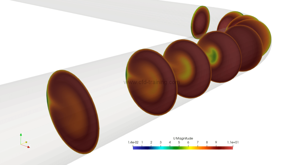
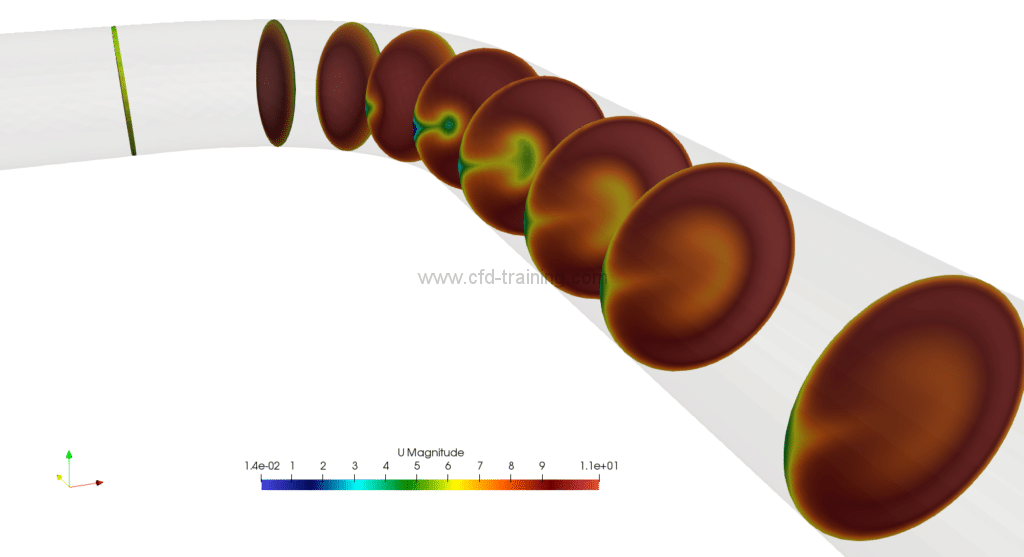
Figure 3 : Velocity field (m/s) cut plane
Horizontal and vertical velocity distribution
The horizontal velocity profiles are located in the model symmetry plane while the vertical profiles are perpendicular to the symmetry plane and located at pipe center. The profiles are marked from the distances z ‘and z and the angle phi shown in Figure 1.
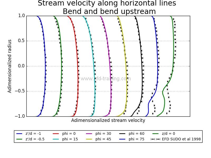
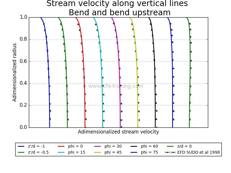
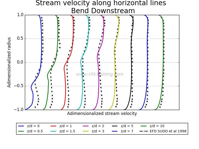
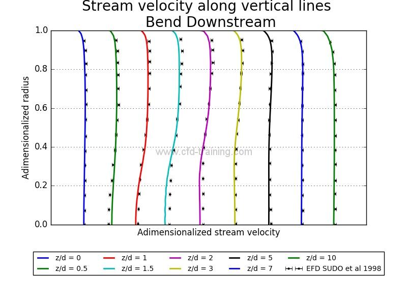
Figure 4 : Numerical/Experimental comparison of spatial mean velocity distribution
